---
title: "Session 11"
description: "Optimal Binary Search Tree"
image: "https://syntax.theether.in/og.png"
---

> Documentation Index
> Fetch the complete documentation index at: https://syntax.theether.in/llms.txt
> Use this file to discover all available pages before exploring further.

# Session 11

This session covers the optimal binary search tree problem. A normal binary search tree only depends on key order, but an optimal BST also considers how frequently each key is searched so that the expected search cost is minimized.

## Objectives

- Understand optimal binary search tree construction.
- Determine the minimum expected search cost.
- Show the final tree structure for the given key probabilities/frequencies.

## Concept

An optimal binary search tree minimizes the expected search cost when keys have different search probabilities. Frequently searched keys should appear closer to the root when that reduces total weighted path cost.

### Dynamic Programming Idea

For each key range, try each key as root and choose the root that gives minimum expected cost.

```text
cost[i][j] = min(cost[i][r-1] + cost[r+1][j] + sum(freq[i..j]))
```

where `r` ranges from `i` to `j`.

## Question 1

### Problem Statement

Determine the cost and structure of an optimal binary search tree for a set of `n = 7` keys with the given properties. Show the step-by-step process.

| i | 0 | 1 | 2 | 3 | 4 | 5 | 6 | 7 |
|---|---|---|---|---|---|---|---|---|
| $p_i$ | | 0.04 | 0.06 | 0.08 | 0.02 | 0.10 | 0.12 | 0.14 |
| $q_i$ | 0.06 | 0.06 | 0.06 | 0.06 | 0.05 | 0.05 | 0.05 | 0.05 |

### Explanation

#### Optimal Tree Structure

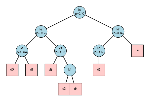
For `n = 7` keys with the given probabilities, the minimum expected search cost is 3.20.

<img src="/216-sc1-ss11-1.png" class="rounded-xl mt-5"/>

### Step-by-Step 

The OBST problem is solved using the standard CLRS dynamic programming approach. We maintain three tables:

- `e[i][j]`: Expected search cost for keys $k_i$ to $k_j$
- `w[i][j]`: Sum of probabilities in the subtree (keys + dummy keys)
- `root[i][j]`: Index of the root key that minimizes `e[i][j]`

#### Recurrence Relations

- Base Case: $`e[i][i-1] = q_{i-1} and w[i][i-1] = q_{i-1}`$ for i = 1 to n+1
- Weight Update: $`w[i][j] = w[i][j-1] + p_j + q_j`$
- Cost Update: $`e[i][j] = min_{r=i..j} { e[i][r-1] + e[r+1][j] } + w[i][j]`$

#### Table Initialization

```sh
e[1][0] = 0.06, e[2][1] = 0.06, e[3][2] = 0.06, e[4][3] = 0.06
e[5][4] = 0.05, e[6][5] = 0.05, e[7][6] = 0.05, e[8][7] = 0.05
w[i][i-1] = e[i][i-1]
```

#### Filling Tables (Length l = 1 to 7)

We iterate over subtree lengths `l`, then start index `i`, compute `j = i + l - 1`, calculate `w[i][j]`, and try every possible root `r` between `i` and `j`.

Example for `l=1, i=1, j=1`:

- `w[1][1] = w[1][0] + p_1 + q_1 = 0.06 + 0.04 + 0.06 = 0.16`
- `e[1][1] = e[1][0] + e[2][1] + w[1][1] = 0.06 + 0.06 + 0.16 = 0.28`
- `root[1][1] = 1`

Repeating this for all `l` yields the final tables:

| `i \ j` | 1 | 2 | 3 | 4 | 5 | 6 | 7 |
|---------|---|---|---|---|---|---|---|
| 1 | 0.28 | 0.62 | 1.02 | 1.38 | 1.87 | 2.50 | 3.20 | 
| 2 |      | 0.30 | 0.68 | 0.96 | 1.45 | 2.02 | 2.68 |
| 3 |      |      | 0.32 | 0.60 | 1.07 | 1.54 | 2.20 |
| 4 |      |      |      | 0.26 | 0.60 | 1.06 | 1.61 |
| 5 |      |      |      |      | 0.32 | 0.75 | 1.25 |
| 6 |      |      |      |      |      | 0.34 | 0.81 |
| 7 |      |      |      |      |      |      | 0.36 |

#### Tree Reconstruction

Starting from root[1][7] = 5, we recursively find subtrees:
- `root[1][4] = 2` → `k2` is left child of `k5`
- `root[6][7] = 7` → `k7` is right child of `k5`
- Continue recursively until all `root[i][j]` and base dummy keys are placed.

### Implementation

### Python

```python title="binary-search.py" file=<rootDir>/public/code/mcs-216/section-1/session-11/1/1.py 

```
### C

```c title="binary-search.c" file=<rootDir>/public/code/mcs-216/section-1/session-11/1/1.c 

```
### Rust

```rust title="binary-search.rs" file=<rootDir>/public/code/mcs-216/section-1/session-11/1/1.rs

```

### Sample Output

```sh
Optimal Expected Cost: 3.1200

Tree Structure:
L -> k5 (p=0.10)
L -> k2 (p=0.06)
    L -> k1 (p=0.04)
        L -> d0 (q=0.06)
        R -> d1 (q=0.06)
    R -> k3 (p=0.08)
        L -> d2 (q=0.06)
        R -> k4 (p=0.02)
            L -> d3 (q=0.06)
            R -> d4 (q=0.05)
R -> k7 (p=0.14)
    L -> k6 (p=0.12)
        L -> d5 (q=0.05)
        R -> d6 (q=0.05)
    R -> d7 (q=0.05)
```

## Question 2

### Problem Statement

Determine the cost and structure of an optimal binary search tree for a set of `n = 5` keys with the given properties. Show the step-by-step process.

| i | 0 | 1 | 2 | 3 | 4 | 5 |
|---|---|---|---|---|---|---|
| $p_i$ | | 0.15 | 0.10 | 0.05 | 0.10 | 0.20| 
| $q_i$ | 0.05 | 0.10 | 0.05 | 0.05 | 0.05 | 0.10| 

### Answer

#### Dynamic Programming Formulation

We use three $O(n^2)$ tables:
- `e[i][j]`: Expected search cost for keys $k_i \dots k_j$
- `w[i][j]`: Probability weight of subtree $i \dots j$
- `root[i][j]`: Index of the optimal root for subtree $i \dots j$

#### **Recurrence Relations:**
1. **Base Case:** $`e[i][i-1] = q_{i-1}$, $w[i][i-1] = q_{i-1}`$
2. **Weight Update:** $`w[i][j] = w[i][j-1] + p_j + q_j`$
3. **Cost Update:** $`e[i][j] = \min_{r=i}^{j} { e[i][r-1] + e[r+1][j] } + w[i][j]`$

### Step-by-Step DP Calculation

#### Step 1: Base Cases (`l = 0`)
| `i` | `e[i][i-1]` | `w[i][i-1]` |
|:---:|:-----------:|:-----------:|
| 1   | 0.05        | 0.05        |
| 2   | 0.10        | 0.10        |
| 3   | 0.05        | 0.05        |
| 4   | 0.05        | 0.05        |
| 5   | 0.05        | 0.05        |
| 6   | 0.10        | 0.10        |

#### Step 2: Chain Length `l = 1`
| `i` | `j` | `w[i][j]` | `e[i][j]` | `root[i][j]` | Calculation (`min` expression) |
|:---:|:---:|:---------:|:---------:|:------------:|:-------------------------------|
| 1   | 1   | 0.30      | **0.45**  | 1            | `0.05 + 0.10 + 0.30`           |
| 2   | 2   | 0.25      | **0.40**  | 2            | `0.10 + 0.05 + 0.25`           |
| 3   | 3   | 0.15      | **0.25**  | 3            | `0.05 + 0.05 + 0.15`           |
| 4   | 4   | 0.20      | **0.30**  | 4            | `0.05 + 0.05 + 0.20`           |
| 5   | 5   | 0.35      | **0.50**  | 5            | `0.05 + 0.10 + 0.35`           |

#### Step 3: Chain Length `l = 2`
| `i` | `j` | `w[i][j]` | `e[i][j]` | `root[i][j]` | Best `r` & Calculation |
|:---:|:---:|:---------:|:---------:|:------------:|:-----------------------|
| 1   | 2   | 0.45      | **0.90**  | 1            | `r=1: 0.05 + 0.40 + 0.45` |
| 2   | 3   | 0.35      | **0.70**  | 2            | `r=2: 0.10 + 0.25 + 0.35` |
| 3   | 4   | 0.30      | **0.60**  | 4            | `r=4: 0.25 + 0.05 + 0.30` |
| 4   | 5   | 0.50      | **0.90**  | 5            | `r=5: 0.30 + 0.10 + 0.50` |

#### Step 4: Chain Length `l = 3`
| `i` | `j` | `w[i][j]` | `e[i][j]` | `root[i][j]` | Best `r` & Calculation |
|:---:|:---:|:---------:|:---------:|:------------:|:-----------------------|
| 1   | 3   | 0.55      | **1.25**  | 2            | `r=2: 0.45 + 0.25 + 0.55` |
| 2   | 4   | 0.50      | **1.20**  | 2            | `r=2: 0.10 + 0.60 + 0.50` |
| 3   | 5   | 0.60      | **1.30**  | 5            | `r=5: 0.60 + 0.10 + 0.60` |

#### Step 5: Chain Length `l = 4`
| `i` | `j` | `w[i][j]` | `e[i][j]` | `root[i][j]` | Best `r` & Calculation |
|:---:|:---:|:---------:|:---------:|:------------:|:-----------------------|
| 1   | 4   | 0.70      | **1.75**  | 2            | `r=2: 0.45 + 0.60 + 0.70` |
| 2   | 5   | 0.80      | **2.00**  | 4            | `r=4: 0.70 + 0.50 + 0.80` |

#### Step 6: Chain Length `l = 5` (Full Tree)
| `i` | `j` | `w[i][j]` | `e[i][j]` | `root[i][j]` | Best `r` & Calculation |
|:---:|:---:|:---------:|:---------:|:------------:|:-----------------------|
| 1   | 5   | 1.00      | **2.75**  | 2            | `r=2: 0.45 + 1.30 + 1.00` |

---

### Final DP Tables

#### Expected Cost Table `e[i][j]`
| `i\j` | 1    | 2    | 3    | 4    | 5    |
|:-----:|:----:|:----:|:----:|:----:|:----:|
| **1** | 0.45 | 0.90 | 1.25 | 1.75 | **2.75** |
| **2** | —    | 0.40 | 0.70 | 1.20 | 2.00   |
| **3** | —    | —    | 0.25 | 0.60 | 1.30   |
| **4** | —    | —    | —    | 0.30 | 0.90   |
| **5** | —    | —    | —    | —    | 0.50   |

#### Optimal Root Table `root[i][j]`
| `i\j` | 1 | 2 | 3 | 4 | 5 |
|:-----:|:-:|:-:|:-:|:-:|:-:|
| **1** | 1 | 1 | 2 | 2 | **2** |
| **2** | — | 2 | 2 | 2 | 4   |
| **3** | — | — | 3 | 4 | 5   |
| **4** | — | — | — | 4 | 5   |
| **5** | — | — | — | — | 5   |

### Optimal Tree Structure

<img src="/216-sc1-ss11-1.png" class="rounded-xl mt-5"/>

### Implementation

### Python

```python title="binary-search.py" file=<rootDir>/public/code/mcs-216/section-1/session-11/2/2.py 

```
### C

```c title="binary-search.c" file=<rootDir>/public/code/mcs-216/section-1/session-11/2/2.c 

```
### Rust

```rust title="binary-search.rs" file=<rootDir>/public/code/mcs-216/section-1/session-11/2/2.rs

```

### Sample Output

```sh
Optimal Expected Cost: 2.7500

Tree Structure:
R -> k2 (p=0.10)
L -> k1 (p=0.15)
    L -> d0 (q=0.05)
    R -> d1 (q=0.10)
R -> k5 (p=0.20)
    L -> k4 (p=0.10)
        L -> k3 (p=0.05)
            L -> d2 (q=0.05)
            R -> d3 (q=0.05)
        R -> d4 (q=0.05)
    R -> d5 (q=0.10)
```

## Question 3

### Problem Statement

Implement the optimal binary search tree algorithm on your system and study the performance of the algorithm on different problem instances

Source: https://syntax.theether.in/mcs-216/section-1/session-11/index.mdx